Multi-fidelity classification
Published:
Multi-fidelity classification using Gaussian processes: Accelerating the prediction of large-scale computational models
Francisco Sahli Costabal, Paris Perdikaris, Ellen Kuhl and Daniel E. Hurtado
This post explain the basic usage of a Gaussian process multi-fidelity classifier in pyMC3 that we developed in our article in Computer Methods in Applied Mechanics and Engineering. The source code can be found here. The motivation for this work is that there are many computational models that predict a binary output (success/fail) and can be very expensive to run. In some cases there are inexpensive approximations that can be run in a fraction of the time. Combining the output of these models to predict the output of the high fidelity, expensive model is the whole area of research of multi-fidelity methods. However, all current methods focus on continuous variables, so here we introduce a Gaussian process classifier to handle the classification case of binary variables. All the details can be found in the article:
@article{SahliCostabal2019,
title = "Multi-fidelity classification using Gaussian processes: Accelerating the prediction of large-scale computational models",
journal = "Computer Methods in Applied Mechanics and Engineering",
volume = "357",
pages = "112602",
year = "2019",
issn = "0045-7825",
doi = "https://doi.org/10.1016/j.cma.2019.112602",
url = "http://www.sciencedirect.com/science/article/pii/S0045782519304785",
author = "Francisco Sahli Costabal and Paris Perdikaris and Ellen Kuhl and Daniel E. Hurtado"
}
In the package, there are four types of classifiers available:
- Gaussian process classifier:
GPclassifier - Sparse Gaussian process classifier:
SGPclassifier - Multi-fidelity classifier:
MFGPclassifier - Sparse multi-fidelity classifier:
SMFGPclassifier
All the classifiers have the following methods:
classifier.create_model(): to initialize the model.classifier.sample_model(): to perform the inference using NUTS. This is tipically the step that takes longer.classifier.sample_predictive(X_star, n_samples = 100): generate n_samples samples at the locations X_star for the latent (high fidelity) Gaussian process. To obtain a single prediction for each point use:from GPmodels import invlogit y_star = invlogit(classifier.sample_predictive(X_star, n_samples = 100).mean(0))classifier.active_learning(N = 15, plot = False): active learning option, where the next point is adaptively sample to improve accuracy.classifier.plot(): plot the classifier and the active learning distribution. Works only for 2D examples.classifier.test_model(): compute the accuracy at theX_testlocations given in the initialization
Dependencies:
- pyMC3: https://docs.pymc.io
- pyDOE:
pip install pydoe - matplotlib, numpy, scipy
Demo
%load_ext autoreload
%autoreload 2

import numpy as np
import matplotlib.pyplot as plt
from pyDOE import lhs
from GPmodels import GPclassifier, MFGPclassifier, SMFGPclassifier, SGPclassifier
from scipy.cluster.vq import kmeans

plt.rcParams['image.cmap'] = 'coolwarm'
np.random.seed(2)
Define the functions used in the first example of the publication
def low_fidelity(X):
    return (0.45 + np.sin(2.2*X[:,0]*np.pi)/2.5 - X[:,1]) > 0

def high_fidelity(X):
    return ( 0.5 + np.sin(2.5*X[:,0]*np.pi)/3 - X[:,1]) > 0

def low_fidelity_boundary(X):
    return (0.45 + np.sin(2.2*X[:,0]*np.pi)/2.5)

def high_fidelity_boundary(X):
    return (0.5 + np.sin(2.5*X[:,0]*np.pi)/3)
Generate some data
# upper and lower bounds of the data. Used for normalization
# and to set the parameter space in the active learning case
lb = np.array([0,0])
ub = np.array([1,1])

N_L = 50 # number of low fidelity points
N_H = 10 # number of high fidelity points
X_L= lhs(2,N_L) # generate data with a Latin hypercube desing
labels_low = low_fidelity(X_L)
Y_L = 1.0*labels_low

# to generate the high fidelity data we choose some points
# from both of classes in the low fidelity data
ind1 = np.where(Y_L > 0)[0]
ind0 = np.where(Y_L == 0)[0]

X_H1 = X_L[np.random.choice(ind1, N_H/2, replace = False)]
X_H0 = X_L[np.random.choice(ind0, N_H/2, replace = False)]

X_H = np.concatenate((X_H1, X_H0))

labels_high = high_fidelity(X_H)
Y_H = 1.0*labels_high

X_test = lhs(2,1000) # to test the accuracy
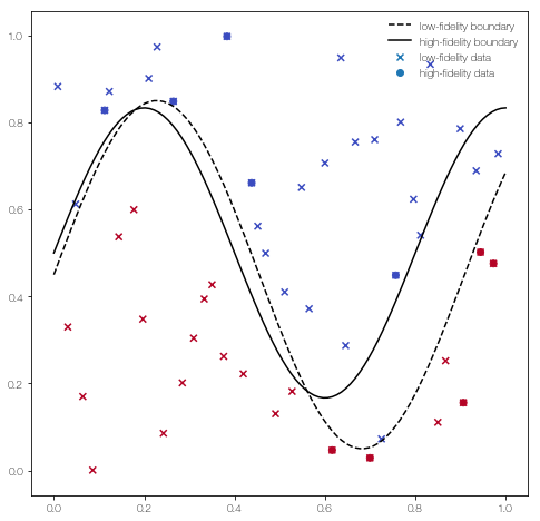
… and plot it
fig = plt.figure()
fig.set_size_inches((8,8))

plt.scatter(X_L[:,0], X_L[:,1], c = Y_L, marker = 'x', label = 'low-fidelity data')
plt.scatter(X_H[:,0], X_H[:,1], c = Y_H, label = 'high-fidelity data')

x = np.linspace(0, 1, 100)[:,None]

plt.plot(x, low_fidelity_boundary(x), 'k--', label = 'low-fidelity boundary')
plt.plot(x , high_fidelity_boundary(x), 'k', label = 'high-fidelity boundary')

plt.legend(frameon = False)
<matplotlib.legend.Legend at 0x1c22036150>
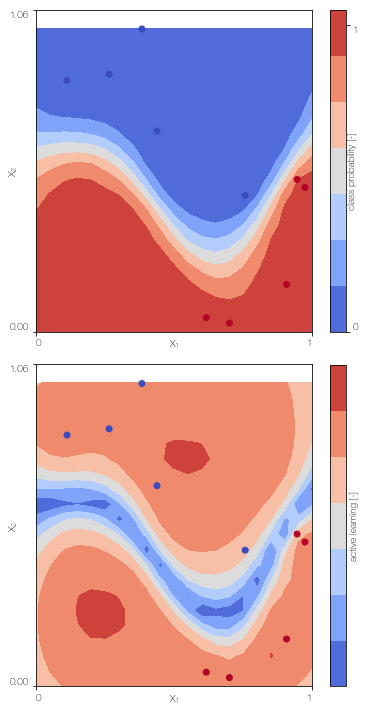
Gaussian process classifier
Train the single fidelity classifier on the low fidelity data
GPc = GPclassifier(X_L, Y_L, lb, ub, low_fidelity, X_test = X_test)
# the low_fidelity function is needed for active learning.
# otherwise set to None
GPc.create_model()
GPc.sample_model()
Auto-assigning NUTS sampler...
Initializing NUTS using jitter+adapt_diag...
/Users/fsc/anaconda/envs/ml/lib/python2.7/site-packages/theano/tensor/basic.py:6592: FutureWarning: Using a non-tuple sequence for multidimensional indexing is deprecated; use `arr[tuple(seq)]` instead of `arr[seq]`. In the future this will be interpreted as an array index, `arr[np.array(seq)]`, which will result either in an error or a different result.
  result[diagonal_slice] = x
Multiprocess sampling (2 chains in 4 jobs)
NUTS: [fp_rotated_, eta_L, l_L]
The number of effective samples is smaller than 25% for some parameters.
GPc.plot() # only works for 2D
100%|██████████| 500/500 [00:38<00:00, 12.93it/s]
Sparse Gaussian process classifier
Train the sparse single fidelity classifier on the low fidelity data
X_Lu = kmeans(X_L,30)[0] # k-means clustering to obtain the position of the inducing points

SGPc = SGPclassifier(X_L, Y_L, X_Lu, lb, ub, low_fidelity, X_test = X_test)
# the low_fidelity function is needed for active learning.
# otherwise set to None
SGPc.create_model()
SGPc.sample_model()
Auto-assigning NUTS sampler...
Initializing NUTS using jitter+adapt_diag...
Multiprocess sampling (2 chains in 4 jobs)
NUTS: [fp_rotated_, u_rotated_, eta_L, l_L]
The number of effective samples is smaller than 25% for some parameters.
SGPc.plot() # only works for 2D
100%|██████████| 500/500 [00:49<00:00, 10.03it/s]
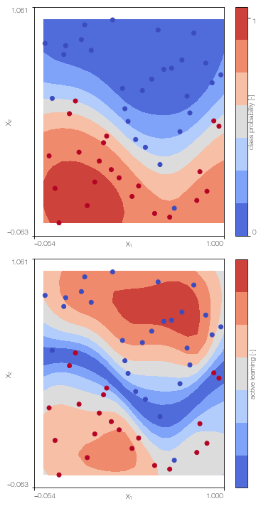
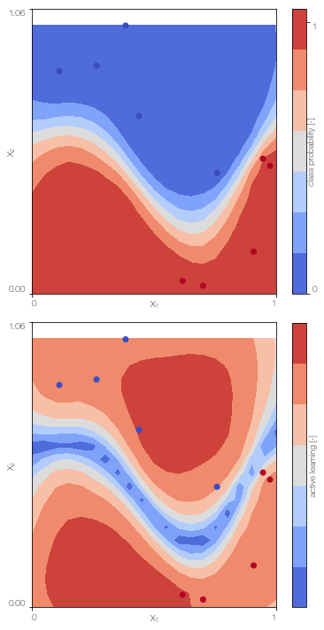
Multi-fidelity Gaussian process classifier
Train the multi-fidelity classifier on low fidelity and high fidelity data
MFGPc = MFGPclassifier(X_L, Y_L, X_H, Y_H, lb, ub, high_fidelity, X_test = X_test)
# the high_fidelity function is needed for active learning.
# otherwise set to None
MFGPc.create_model()
MFGPc.sample_model()
Auto-assigning NUTS sampler...
Initializing NUTS using jitter+adapt_diag...
Multiprocess sampling (2 chains in 4 jobs)
NUTS: [fp_rotated_, eta_H, delta, l_H, eta_L, l_L]
There was 1 divergence after tuning. Increase `target_accept` or reparameterize.
The number of effective samples is smaller than 25% for some parameters.
MFGPc.plot()
100%|██████████| 500/500 [00:40<00:00, 12.22it/s]
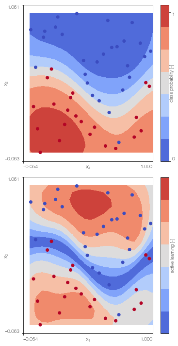
Sparse ulti-fidelity Gaussian process classifier
Train the sparse multi-fidelity classifier on low fidelity and high fidelity data
X_Lu = kmeans(X_L,30)[0] # k-means clustering to obtain the position of the inducing points
X_Hu = X_H # we use the high fidelity points as inducing points as well because there only 10.

SMFGPc = SMFGPclassifier(X_L, Y_L, X_H, Y_H, X_Lu, X_Hu, lb, ub, high_fidelity, X_test = X_test)
SMFGPc.create_model()
SMFGPc.sample_model()
Auto-assigning NUTS sampler...
Initializing NUTS using jitter+adapt_diag...
Multiprocess sampling (2 chains in 4 jobs)
NUTS: [fp_rotated_, u_rotated_, eta_H, delta, l_H, eta_L, l_L]
There was 1 divergence after tuning. Increase `target_accept` or reparameterize.
There was 1 divergence after tuning. Increase `target_accept` or reparameterize.
The number of effective samples is smaller than 25% for some parameters.
SMFGPc.plot()
100%|██████████| 500/500 [01:32<00:00, 6.08it/s]